Feature selection

Morphological profile features often exhibit strong correlation structures. This can obfuscate downstream analysis - such as asking “what features most often changed between treatment and control? Similarly, features that are associated with platemap- or batch effects can hinder meaningful analysis. For this reason, scmorph integrates ways to remove features that are redundant or associated with known confounders.

Removing correlations

# Ignore warnings
import warnings

warnings.filterwarnings("ignore", category=RuntimeWarning)

import scmorph as sm
import matplotlib.pyplot as plt

adata = sm.datasets.rohban2017_minimal()
adata.shape

(12352, 1687)

This example dataset has 1687 features, many of which will be at least partly redundant. scmorph makes removing redunant features easy:

adata_filtered_pearson = sm.pp.select_features(adata, method="pearson", copy=True)
adata_filtered_pearson.shape

(12352, 1455)

Behind the scenes, this is what happens:

1. Correlate all features with each other

2. For any feature pair with correlation coefficient > threshold (0.9 by default), remove one of the features. To decide which one, check which of the two features has the higher correlation with all other features.

By varying the treshold, we can be more or less stringent in our filtering.

adata_filtered_pearson = sm.pp.select_features(adata, method="pearson", cor_cutoff=0.8, copy=True)
adata_filtered_pearson.shape

(12352, 1306)

Likewise, we can use other correlation coefficients that may be more suitable for morphological features, which do not always follow normal distributions.

adata_filtered_spearman = sm.pp.select_features(adata, method="spearman", cor_cutoff=0.8, copy=True)
adata_filtered_spearman.shape

(12352, 1295)

We can also subset the data before performing this correlation filtering, which can help speed up processing speeds for large datasets. For example, if we only want to use 3000 cells while estimating correlations, we can use n_obs as below. Note that, because we are not using the full data while computing correlation coefficients, this can influence the number of features retained.

adata_filtered_spearman = sm.pp.select_features(
    adata, method="spearman", cor_cutoff=0.8, copy=True, n_obs=3000
)
adata_filtered_spearman.shape

(12352, 1293)

scmorph also integrates an adapted version of the Chatterjee correlation coefficient, based on work by Lin and Han (2021). While it is slower to compute than the other correlation coefficients, it makes fewer assumptions and can find correlations that may be missed by other coefficients of correlation.

adata_filtered_spearman = sm.pp.select_features(
    adata, method="chatterjee", cor_cutoff=0.7, copy=True, n_obs=1000
)
adata_filtered_spearman.shape

(12352, 1477)

Note that select_features also does some additional filtering behind the scenes. Specifically, it removes features with very low variance. Features affected by this filter are usually not informative and can be safely removed. You can see which features are affected by this filter after running the select_features function by looking at the corresponding data in var:

adata.var["qc_pass_var"].value_counts()

True     1585
False     102
Name: qc_pass_var, dtype: int64

To see some example features that do not pass this variance threshold, you could use the following:

adata.var.query("qc_pass_var == False").sample(5)

	Object	Module	feature_1	feature_2	feature_3	feature_4	qc_pass_var
Cells_Correlation_Costes_RNA_Mito	Cells	Correlation	Costes	RNA	Mito	NaN	False
Cells_Correlation_Costes_ER_RNA	Cells	Correlation	Costes	ER	RNA	NaN	False
Cytoplasm_Intensity_MeanIntensityEdge_DNA	Cytoplasm	Intensity	MeanIntensityEdge	DNA	NaN	NaN	False
Nuclei_AreaShape_Zernike_9_7	Nuclei	AreaShape	Zernike	9	7	NaN	False
Cells_Intensity_MADIntensity_DNA	Cells	Intensity	MADIntensity	DNA	NaN	NaN	False

Removing confounded features

In this second part, let’s try to remove features that are associated with the plate ID. Note there is also a dedicated tutorial on batch correction, which covers this topic in more detail. However, the methods discussed here can also be applied to removing row- or column-effects.

Once again, we will start with the same minimal dataset used above. But now we will use the Kruskal Wallis statistic to detect features that are associated with the plate ID.

To find features that may be affected by batch effects, we can run the kruskal_test function.

sm.pp.kruskal_test(adata, test_column="Image_Metadata_Plate")

AnnData object with n_obs × n_vars = 12352 × 1687
    obs: 'TableNumber', 'ImageNumber', 'ObjectNumber', 'Image_Metadata_Plate', 'Image_Metadata_Site', 'Image_Metadata_Well', 'PUBLICID', 'TA_GeneID', 'Duplicate.ORFs', 'TARGETTRANS', 'Activator.Inhibitor', 'CONSTRUCTNAME', 'ISMUTANT', 'TARGETGENE', 'TA_REF.vs..DLBCL', 'ReferencePathway.Process'
    var: 'Object', 'Module', 'feature_1', 'feature_2', 'feature_3', 'feature_4', 'qc_pass_var'
    uns: 'kruskal_test'
    obsm: 'inter_cell_features', 'intra_cell_features'
    varm: 'pearson', 'spearman', 'chatterjee'

This function stores information about features’ association in the uns slot:

adata.uns["kruskal_test"]["Image_Metadata_Plate"].head()

	feature	statistic	pvalue
0	Nuclei_AreaShape_Area	35.128770	4.370841e-07
1	Nuclei_AreaShape_Compactness	34.413338	6.130122e-07
2	Nuclei_AreaShape_Eccentricity	44.511616	5.022926e-09
3	Nuclei_AreaShape_EulerNumber	3.429444	4.886873e-01
4	Nuclei_AreaShape_FormFactor	15.949369	3.087861e-03

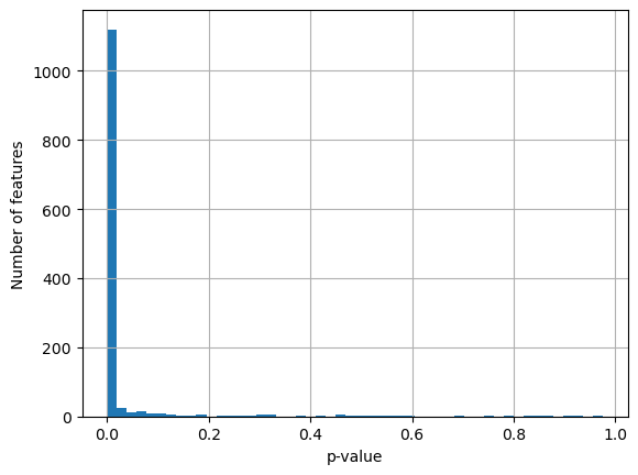
Oftentimes the p-value obtained from the KW test is overly harsh - most features are marked as significantly associated with plate IDs, while the KW statistics are mostly not as extreme as the p-value would suggest.

adata.uns["kruskal_test"]["Image_Metadata_Plate"]["pvalue"].hist(bins=50)
plt.xlabel("p-value")
plt.ylabel("Number of features")
plt.show()

adata.uns["kruskal_test"]["Image_Metadata_Plate"]["statistic"].hist(bins=50)
plt.xlabel("KW statistic")
plt.ylabel("Number of features")
plt.show()

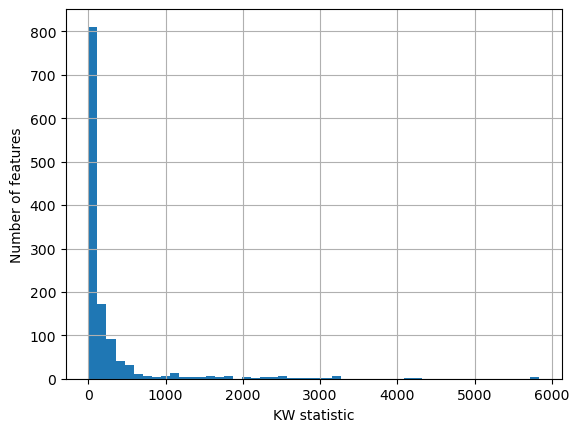
So we can instead choose to filter features based on how extreme their KW statistic is. To do so, we can use the kruskal_filter function which marks a feature as associated with batches if its KW statistic is more than one median absolute deviation away from the median of all other features’ KW statistics. Applying this here, this removes about half of the features as associated with plate IDs.

adata_filtered = sm.pp.kruskal_filter(adata, "Image_Metadata_Plate")
adata_filtered.shape

(12352, 796)

You could think of applying the same principle to row or column IDs to remove features associated with platemap effects.

Taken together, with scmorph you can mitigate some of the problems that morphological profiling experiments hold - such as batch effects and heavy correlation structures.