Batch effects

This tutorial will describe a basic workflow to

1. Load in an example dataset

2. Identify batch effects in morphological profiling experiments

3. Remove those effects

Along the way, we will describe the basic anatomy of AnnData objects, which form the backbone of the data structure that scmorph uses. For more on AnnData objects, please refer to the package’s documentation.

We will be using a minimal example dataset published in Rohban et al. (2017). In it, the authors performed overexpression experiments of genes. To start our investigation of this data, let’s load it!

# Load scmorph
import scmorph as sm
import matplotlib.pyplot as plt

# Load in a subset of the Rohban data
# To load in the full dataset, you may use sm.datasets.rohban2017()
# but note that this will download the dataset from the internet,
# occupying ~8Gb of disk space.
adata = sm.datasets.rohban2017_minimal()

In AnnData objects, rows represent cells and columns represent features. AnnData compartmentalises the data into different slots. For example, the cell by feature matrix is stored in the .X slot. That means that if you wish to access it, you would use adata.X. Similarly, metadata about your observations (i.e. cells) is stored in .obs, and metadata about variables (i.e. features) is found in .var. Let’s test this by seeing what metadata is attached to our cells.

adata.obs

	TableNumber	ImageNumber	ObjectNumber	Image_Metadata_Plate	Image_Metadata_Site	Image_Metadata_Well	PUBLICID	TA_GeneID	Duplicate.ORFs	TARGETTRANS	Activator.Inhibitor	CONSTRUCTNAME	ISMUTANT	TARGETGENE	TA_REF.vs..DLBCL	ReferencePathway.Process
0	7a6fb88c134a0004353010f30dba103c	1	1	41744	1	a01	0	NaN	NaN	NaN	NaN	NaN	NaN	NaN	NaN	NaN
1	7a6fb88c134a0004353010f30dba103c	1	2	41744	1	a01	0	NaN	NaN	NaN	NaN	NaN	NaN	NaN	NaN	NaN
2	7a6fb88c134a0004353010f30dba103c	1	3	41744	1	a01	0	NaN	NaN	NaN	NaN	NaN	NaN	NaN	NaN	NaN
3	7a6fb88c134a0004353010f30dba103c	1	4	41744	1	a01	0	NaN	NaN	NaN	NaN	NaN	NaN	NaN	NaN	NaN
4	7a6fb88c134a0004353010f30dba103c	1	5	41744	1	a01	0	NaN	NaN	NaN	NaN	NaN	NaN	NaN	NaN	NaN
...	...	...	...	...	...	...	...	...	...	...	...	...	...	...	...	...
77417-4	dc859c7c96dd79087b6463aa30f69dd6	1116	49	41757	9	f04	BRDN0000464847	1050.0	duplicate-Cat2	NM_004364.3	0	ORF023754.1_TRC304.1	0.0	CEBPA	TA_REF	Transcription Factors
77418-4	dc859c7c96dd79087b6463aa30f69dd6	1116	50	41757	9	f04	BRDN0000464847	1050.0	duplicate-Cat2	NM_004364.3	0	ORF023754.1_TRC304.1	0.0	CEBPA	TA_REF	Transcription Factors
77419-4	dc859c7c96dd79087b6463aa30f69dd6	1116	51	41757	9	f04	BRDN0000464847	1050.0	duplicate-Cat2	NM_004364.3	0	ORF023754.1_TRC304.1	0.0	CEBPA	TA_REF	Transcription Factors
77420-4	dc859c7c96dd79087b6463aa30f69dd6	1116	52	41757	9	f04	BRDN0000464847	1050.0	duplicate-Cat2	NM_004364.3	0	ORF023754.1_TRC304.1	0.0	CEBPA	TA_REF	Transcription Factors
77421-4	dc859c7c96dd79087b6463aa30f69dd6	1116	53	41757	9	f04	BRDN0000464847	1050.0	duplicate-Cat2	NM_004364.3	0	ORF023754.1_TRC304.1	0.0	CEBPA	TA_REF	Transcription Factors

12352 rows × 16 columns

Information about which gene was overexpressed can be found in the TARGETGENE column. For untreated cells, the published data contained missing values. Let’s fill them in with UNTREATED to mark negative controls.

adata.obs["TARGETGENE"] = adata.obs["TARGETGENE"].astype(str).replace("nan", "UNTREATED")

Next up: cleaning the data a bit further.

The observations the Rohban et al., 2017, provide are not all complete: some cells did not have all features measured. Our standard workflow will start by removing those cells.

# How many cells are there before filtering?
print(adata.shape)

# Remove cells with missing values
sm.pp.drop_na(adata)

# How many cells are there after filtering?
print(adata.shape)

(12352, 1687)
(12286, 1687)

Next, we may wish to remove any batch effects that may be present. We will use the controls on each plate to normalize. Let’s first look if any batch effects are present by checking the average actin/Golgi/membrane intensity across plates in control cells.

Note: we check batch effects on control cells only to ignore any treatment-related differences between plates.

# Subset AnnData object to only include untreated cells
adata_ctrl = adata[adata.obs["TARGETGENE"] == "UNTREATED"]

# Use scmorph to plot the cumulative density of the mean AGP intensity
sm.pl.cumulative_density(
    adata_ctrl,
    "Cells_Intensity_MeanIntensity_AGP",
    color="Image_Metadata_Plate",
    xlim=(0.03, 0.08),
    palette="viridis",
    xlabel="Avg. AGP intensity",
)
plt.show()

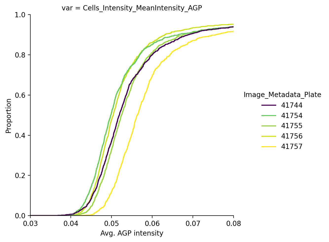
We see that the average AGP intensity differs per plate. We can also see this in PCA space, for example in PC1 the control cells look like this:

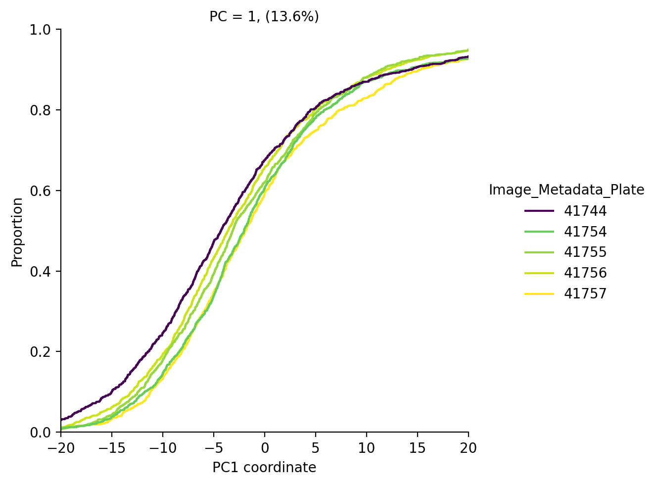
Now that we have confirmed that batch effects are present in this experiment, let’s try to remove them.

adata_corrected = sm.pp.remove_batch_effects(
    adata,
    batch_key="Image_Metadata_Plate",
    treatment_key="TARGETGENE",
    control="UNTREATED",
    copy=True,
)

Computing batch effects...
Removing batch effects...

Did this work in removing batch effects?

adata_ctrl = adata_corrected[adata_corrected.obs["TARGETGENE"] == "UNTREATED"]

sm.pl.cumulative_density(
    adata_ctrl,
    "Cells_Intensity_MeanIntensity_AGP",
    color="Image_Metadata_Plate",
    xlim=(0.03, 0.08),
    palette="viridis",
    xlabel="Avg. AGP intensity",
)
plt.show()

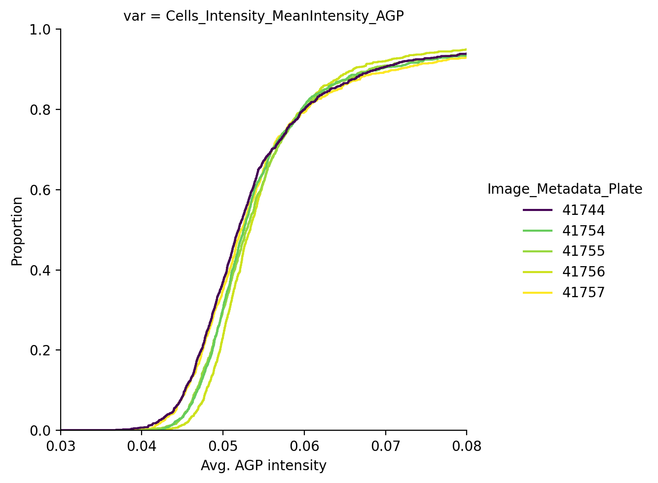
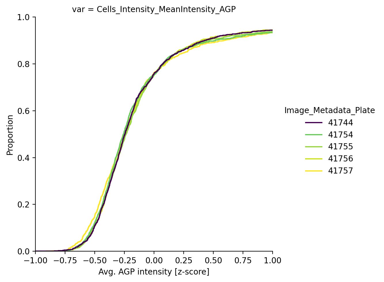
The batch correction technique integrated in scmorph removes the mean batch effect per plate and will thus not lead to all of these lines perfectly overlapping, but the result is better than doing no correction at all. Alternatively, if downstream interpretation of features is not so important, we may instead choose to do per-plate z-scoring.

adata_corrected = adata.copy()

# Perform per-plate z-scoring
sm.pp.scale_by_batch(
    adata_corrected,
    batch_key="Image_Metadata_Plate",
    treatment_key="TARGETGENE",
    control="UNTREATED",
)

adata_ctrl = adata_corrected[adata_corrected.obs["TARGETGENE"] == "UNTREATED"]
sm.pl.cumulative_density(
    adata_ctrl,
    "Cells_Intensity_MeanIntensity_AGP",
    color="Image_Metadata_Plate",
    xlim=(-1, 1),
    palette="viridis",
    xlabel="Avg. AGP intensity [z-score]",
)
plt.show()

This concludes this tutorial, where we learnt how to

1. Load in an example dataset

2. Identify batch effects in morphological profiling experiments

3. Remove those effects